

The Impact of Water Temperature on Oxygen Saturation: A Seasonal Guide
When temperature rises, oxygen flees. Are you ready?
Physics is non-negotiable. As water heats up, its capacity to hold oxygen drops. This seasonal guide shows you how to fight back.
Biological systems depend on dissolved oxygen (DO) to drive metabolic processes and maintain aerobic conditions. When thermal energy increases within a liquid medium, the kinetic energy of gas molecules also rises, leading to a higher rate of escape from the liquid surface. This physical reality dictates the operational parameters of every pond, wastewater lagoon, and aquaculture facility.
Managing these fluctuations requires a precise understanding of gas solubility laws and aeration mechanics. Static systems that perform adequately in cooler months often fail during peak thermal periods. Transitioning from a passive management style to a proactive, data-driven approach is the only way to ensure system stability when environmental conditions become unfavorable.
The Impact of Water Temperature on Oxygen Saturation: A Seasonal Guide
Dissolved oxygen saturation is an inverse function of water temperature. In pure water at sea level, the maximum amount of oxygen that can be held at 0°C is approximately 14.6 mg/L. As the temperature climbs to 30°C, this capacity falls to roughly 7.5 mg/L. This represents a nearly 50% reduction in the available oxygen buffer.
Temperature dictates the saturation ceiling. When a water body reaches 100% saturation at 30°C, it contains significantly less oxygen by mass than the same volume at 15°C. This lower ceiling is critical because the biological oxygen demand (BOD) of the system does not decrease as temperatures rise; in fact, it typically increases. Microorganisms and aquatic life experience accelerated metabolic rates in warmer water, requiring more oxygen even as the water's ability to supply it diminishes.
Seasonal shifts drive these dynamics through thermal stratification. During summer, the upper layer of water (the epilimnion) absorbs solar radiation and becomes less dense. This warm layer floats on top of the cooler, denser bottom water (the hypolimnion). The boundary between them, known as the thermocline or metalimnion, acts as a physical barrier that prevents atmospheric oxygen from reaching the lower depths.
In many systems, this leads to anoxic conditions at the bottom. Bacteria continue to decompose organic matter, stripping oxygen from the hypolimnion until it is completely depleted. This creates a dangerous imbalance where the majority of the water volume is "dead" space, forcing all aerobic life into the thin, warm upper layer.
Real-world applications of this knowledge are found in wastewater treatment and large-scale aquaculture. Engineers must calculate the "Standard Oxygen Transfer Rate" (SOTR) based on the highest expected seasonal temperatures. Designing for average temperatures is a common failure point that leads to system crashes during heatwaves.
How Gas Transfer Mechanics Function in Aquatic Systems
Oxygen enters water primarily through two mechanisms: atmospheric diffusion and photosynthetic byproduct release. In managed systems, mechanical aeration is introduced to accelerate these natural processes. The efficiency of this transfer is governed by Henry’s Law and Fick’s Law of Diffusion.
Henry’s Law states that the amount of dissolved gas in a liquid is proportional to its partial pressure above the liquid. Since oxygen makes up approximately 21% of the atmosphere, the partial pressure at sea level is relatively constant. However, the solubility constant in the equation changes with temperature. As the liquid heats up, the constant decreases, meaning less oxygen can remain in solution at the same atmospheric pressure.
Fick’s Law describes the rate at which gas moves across the air-water interface. This rate depends on the concentration gradient—the difference between the current DO level and the saturation point. When water is far from saturation, oxygen moves in quickly. As it nears saturation, the transfer rate slows to a crawl.
Mechanical aeration maximizes this transfer by increasing two variables: surface area and turbulence.
- Surface Area: Breaking water into small droplets (surface aeration) or air into small bubbles (subsurface diffusion) increases the contact area where gas exchange occurs.
- Turbulence: Moving water ensures that oxygen-rich water at the interface is quickly replaced by oxygen-depleted water from the depths, maintaining a high concentration gradient.
Subsurface systems, or Dynamic Oxygen Injection, utilize diffusers placed at the bottom. As bubbles rise, they not only transfer oxygen but also create a "gas lift" effect. This physical movement of water from the bottom to the top breaks the thermocline and eliminates thermal stratification.
Efficiency Metrics: Understanding SOTE and SAE
Evaluating an aeration system requires objective metrics that move beyond simple horsepower ratings. Two primary standards are used: Standard Oxygen Transfer Efficiency (SOTE) and Standard Aeration Efficiency (SAE).
SOTE measures the percentage of oxygen transferred from the air delivered to the water. It is heavily influenced by bubble size and water depth. Fine-bubble diffusers typically achieve an SOTE of approximately 1.5% to 2.0% per foot of submergence. For example, a diffuser at a depth of 10 feet might achieve a 20% SOTE. Coarse bubbles are less efficient, often falling below 1% per foot, because their larger volume-to-surface-area ratio limits gas exchange.
SAE is a measure of energy efficiency, expressed as pounds of oxygen transferred per horsepower-hour (lbs O2/hp-hr). This metric is critical for calculating operational costs. A system might have high SOTE but require massive amounts of energy to compress air, resulting in a poor SAE.
Engineers use these metrics to size blowers and diffusers. When water temperatures rise, the "Actual Oxygen Transfer Rate" (AOTR) is calculated by adjusting the SOTR for field conditions, including temperature, elevation, and the "alpha" factor (the presence of surfactants or salts that impede gas transfer).
Benefits of High-Efficiency Aeration Systems
Utilizing a scientifically sized aeration system provides measurable advantages over passive management. The most immediate benefit is the stabilization of DO levels during the critical "pre-dawn" window. During the night, photosynthesis stops, but respiration continues, often causing DO to plummet to lethal levels just before sunrise.
Dynamic systems prevent "Summer Stagnation." By maintaining a uniform temperature and oxygen profile throughout the water column, you maximize the usable volume of the pond or tank. This prevents the buildup of toxic gases like hydrogen sulfide and ammonia in the lower depths, which are common side effects of anoxic conditions.
Energy efficiency is another primary driver. High-SOTE systems allow for the use of smaller blowers, significantly reducing monthly utility expenditures. In wastewater applications, aeration often accounts for 50% to 70% of total energy costs. Upgrading to fine-pore diffusers can yield a return on investment within 18 to 24 months through energy savings alone.
Pathogen suppression is a secondary benefit. Many harmful bacteria and parasites thrive in low-oxygen, stagnant environments. Maintaining high DO levels promotes the growth of beneficial aerobic bacteria, which outcompete pathogens and accelerate the breakdown of organic waste.
Challenges and Common Mistakes in Oxygen Management
A frequent error is the "Under-Sizing Trap." Managers often select aeration equipment based on the surface acreage of a pond rather than the volume or the biological load. A shallow, heavily stocked pond requires significantly more aeration than a deep, low-density lake of the same surface area.
Another pitfall is the failure to account for elevation. Atmospheric pressure decreases as altitude increases, which in turn decreases the partial pressure of oxygen. A system that provides 10 lbs of oxygen at sea level will provide significantly less at 5,000 feet. Ignoring this variable leads to chronic under-oxygenation.
Neglecting "BOD Spikes" is a common operational failure. When water temperatures rise, the rate at which bacteria consume organic matter accelerates. This "Biological Oxygen Demand" can outpace the aeration system's capacity, leading to a rapid DO crash. This is especially prevalent after heavy rains, which wash organic debris into the water, or after an algae bloom die-off.
Maintenance neglect is the final major hurdle. Diffusers can become fouled with mineral deposits or biofilms, increasing the backpressure on blowers and reducing SOTE. Failing to monitor blower filters and diffuser membranes leads to a gradual, often unnoticed, decline in system performance.
Limitations: When Standard Aeration May Not Suffice
Mechanical aeration has physical limits defined by the laws of thermodynamics. In extremely high-load environments—such as intensive recirculating aquaculture systems (RAS)—atmospheric air may not contain enough oxygen to meet the demand. In these cases, the concentration gradient becomes the limiting factor.
Environmental constraints also play a role. In very shallow water (less than 4 feet), subsurface diffusers lose most of their efficiency because the bubbles do not have enough "contact time" with the water before reaching the surface. In these scenarios, surface aerators or venturi injectors are often more effective, though they lack the de-stratification power of deep-water systems.
Thermal trade-offs must be considered. Some aeration methods can actually increase water temperature by facilitating heat exchange with the air. In cold-water fisheries, such as trout ponds, aggressive surface aeration during a heatwave can raise the water temperature above the lethal limit for the fish, even if DO levels remain high.
Chemical interference is another limitation. High concentrations of salts, oils, or surfactants change the surface tension of water, creating a "film" that inhibits the transfer of oxygen molecules. This "Alpha Factor" can reduce the efficiency of a diffuser by up to 50%, requiring a much larger system than clean-water calculations would suggest.
Static Summer Stagnation vs. Dynamic Oxygen Injection
The following table compares the two primary states of oxygen management during high-temperature periods.
| Feature | Static Summer Stagnation | Dynamic Oxygen Injection |
|---|---|---|
| Oxygen Distribution | Concentrated in top 2-3 feet | Uniform throughout water column |
| Thermal Profile | Highly stratified (Hot top/Cold bottom) | Destratified (Consistent temp) |
| BOD Processing | Slow; inhibited by anoxia at bottom | Rapid; aerobic bacteria active at all depths |
| Risk of Fish Kill | High (during turnover or pre-dawn) | Low (buffered against fluctuations) |
| Energy Efficiency | N/A (Passive) | High (Calculated SOTE/SAE) |
Dynamic systems are preferred for any application where biological stability is required. Static systems rely on luck and weather patterns, whereas dynamic injection provides a mechanical guarantee of oxygen availability.
Practical Tips for Optimizing Oxygen Levels
Maximizing the efficiency of your aeration system involves more than just turning it on. Fine-tuning the operation can lead to significant gains in both oxygen levels and energy savings.
- Time Your Aeration: If you are running a limited schedule, prioritize the hours between 10:00 PM and 8:00 AM. This is when natural oxygen production stops and respiration peaks.
- Monitor Diffuser Depth: For every foot of depth you gain, you increase the oxygen transfer efficiency. Ensure diffusers are at the deepest points of the basin, provided they are not buried in silt.
- Use Variable Frequency Drives (VFDs): Installing a VFD on your blower allows you to scale the air output based on real-time DO sensor data. This prevents over-aeration and saves electricity during cooler periods.
- Maintain a Clean Surface: Excessive duckweed or surface film blocks atmospheric exchange. Keeping at least 70% of the surface clear improves the natural "gas exchange" capacity of the water.
Regular testing of the "Alpha Factor" in wastewater applications is also recommended. If your water has a low Alpha (less than 0.6), you may need to increase your diffuser density to compensate for the impeded gas transfer.
Advanced Considerations: The Q10 Coefficient and BOD
Serious practitioners must account for the Q10 temperature coefficient. This rule of thumb states that for every 10°C increase in temperature, the rate of chemical and biological reactions doubles. In an aquatic context, this means that if your water warms from 20°C to 30°C, the bacteria in the system will consume oxygen twice as fast.
This creates a "pincer maneuver" on your DO levels: the supply (saturation ceiling) drops while the demand (metabolism) doubles. To account for this, your aeration system should be designed with a "Safety Factor" of at least 2.0 based on peak summer loads.
Advanced systems utilize "Pure Oxygen Supplementation" (POS) to bypass the 21% atmospheric limit. By injecting pure oxygen, you can achieve saturation levels five times higher than what is possible with air. While the cost of oxygen gas is high, the ability to maintain 20+ mg/L of DO in high-density tanks is sometimes the only way to sustain intensive biological processes.
Scaling considerations are also vital. In large lagoons, "Tapered Aeration" is an effective strategy. This involves placing more diffusers at the influent (inlet) end where the organic load and BOD are highest, and fewer diffusers toward the effluent (outlet) where the water is cleaner.
Example Calculation: Sizing for Summer Demand
Consider a 1-million-gallon wastewater lagoon with a BOD load of 500 lbs per day. At a summer temperature of 30°C, we must calculate the required air flow.
First, determine the Actual Oxygen Requirements (AOR). Due to the increased metabolic rate at 30°C, the AOR might be 1.5 times the standard BOD, or 750 lbs O2/day.
Next, factor in the SOTE. If we use fine-bubble diffusers at 10 feet of depth, we can expect an SOTE of approximately 20%. Since air is only 21% oxygen by weight, we need to deliver 5 lbs of air to get 1 lb of oxygen.
Calculation:
1. Total Oxygen needed = 750 lbs.
2. Oxygen available in air = 21% (0.21).
3. Diffuser Efficiency = 20% (0.20).
4. Required Air (lbs) = 750 / (0.21 * 0.20) = 17,857 lbs of air per day.
This weight of air is then converted to Cubic Feet per Minute (CFM) based on the site's elevation and temperature to select the appropriate blower. This rigorous approach ensures the system will not fail during the hottest week of the year.
Final Thoughts
Maintaining dissolved oxygen in rising temperatures is a challenge of managing the gap between falling supply and rising demand. Physics dictates that water will lose its gas-holding capacity as thermal energy increases, leaving the responsibility of oxygenation entirely to mechanical systems and smart management.
Success in this field requires moving away from "rule of thumb" estimates and toward precise calculations of SOTE, SAE, and BOD loading. By understanding the mechanisms of Henry’s Law and the benefits of dynamic injection, operators can build resilient systems that thrive even in the harshest seasonal conditions.
The transition from a passive observer to an active manager starts with data. Regular monitoring of DO and temperature profiles will reveal the hidden stressors in your system, allowing you to apply these technical principles where they are needed most. Experiment with diffuser placement, optimize your blower schedules, and always design for the peak, not the average.